Creating a network, launching and monitoring its training
In this tutorial, we will focus on the definition of a network, then how to train it and monitor its training with TensorBoard.
Creating a network
Generic Unet and MultiScale architectures are available at path/to/plasmanet/NNet/archs

Sketch of UNet
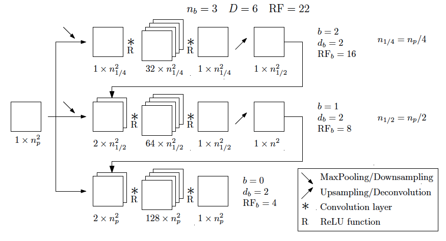
Sketch of MSNet
A new architecture with the desired features can easily be added. For example, you can generate a new .yml file
in this same folder and add the number of desired feature maps per scale. Just note that the scale_0 will correspond
to the scale where the resolution is equal to the input size (\(N_x \times N_y\)), while the highest scale scale_n
matches the images with the lowest resolution (\(\frac{N_x}{2^{n-1}} \times \frac{N_y}{2^{n-1}}\)).
For the Unet networks, all scales are a list containing two lists, where the first matches the left side of the Unet
and the second the right side. Only the bottom scale_n is composed of a single list. The input and output channel
dimensions are hardcoded on scale_0 so make sure that they fit the training pipeline.
UNetModified:
   type: 'UNet'
   args:
      scales:
            scale_0: [[1, 2, 3], [11, 2, 1]]
            scale_1: [[3, 3, 3], [7, 8, 8]]
            scale_2: [3, 4, 4]
      kernel_sizes: 3
MultiScale networks can also be created following the same logic. The scale_0 corresponds to the scale with
the resolution with the original size (\(N_x \times N_y\)). Note that for the MultiScale network, the input field
enters the lowest resolution scale scale_n:
MSNetModified:
   type: 'MSNet'
   args:
      scales:
            scale_0: [2, 2, 2, 3, 2, 2, 1]
            scale_1: [2, 3, 3, 3, 4, 2, 1]
            scale_2: [1, 2, 2, 2, 2, 1]
      kernel_sizes: 3
Further options that can be added on the training yml file.
arch:
   db_file: 'modifed_network.yml'
   name: 'UNetModified'
   args:
      input_res: [101, 401]
      padding_mode: 'custom'
Padding modes can vary between zeros, reflect, replicate, circular or custom. The custom
padding mode correspond to an example of personalized padding used for cylindrical coordinates, where zero padding
is used for the 3D Dirichlet BC and replication padding is used for the axis. The input domain size needs to be declared
as well, as it can be an integer (for squared domains), or a list with size (height, width).
To check the local and global variables of the network, the show_network command shows the receptive field,
number of parameters and depth of the entire network as well as for each individual branch:
show_network -c modified_network.yml
Launching a training
Now that the network and training dataset are created, we simply have to create a Yaml configuration file for the Trainer.
Examples of such can be found in PlasmaNet/NNet.
This file contains multiple blocks, each controlling an aspect of the trainer.
First, we specify the name of the experience which will be used to store the outputs and in TensorBoard as well as the number of GPUs we want to use:
name: 'test/random_8'            # Experience name
n_gpu: 1                         # Number of GPUs to use
Then some global parameters are needed, such as the size of the domain, its coordinate system (cartesian or axisymmetric):
globals:                         # Domain sizes and others, used to compute global attributes
   nnx: 101                      # Number of points in x direction
   nny: 101                      # Number of points in y direction
   xmin: 0.0
   xmax: 1.0e-2
   ymin: 0.0
   ymax: 1.0e-2
   coord: 'cart'                 # Coordinates system ('cart' or 'cyl')
   verbosity: 2                  # Output verbosity level
Now, we specify the network we want to use by directly pointing to the archs database and specifying which network
we want to use in the given database file:
arch:
   db_file: 'unets_ks3_rf100.yml'      # Database file
   name: 'UNet5'                       # Name of the network in the database file
   args:
      input_res: 101                   # Required argument to define the input res of the network
Then, we parametrize the data loader object: its type should correspond to a class defined in PlasmaNet/PlasmaNet/nnet/data,
args should contain all the parameters needed by the class constructor, and the pipe_config specifies if the dataloader
requires the configuration file.
data_loader:
   type: 'PoissonDataLoader'           # Class name of the wanted dataloader
   data_channels: 1                    # Number of data channels
   pipe_config: True                   # Does the dataloader requires the input file?
   args:
      data_dir: 'path/to/your/dataset' # Dataset path
      batch_size: 64
      shuffle: True                    # Do we randomly reorder the dataset?
      validation_split: 0.2            # if float, fraction of the full dataset, if int, length of validation portion
      num_workers: 4                   # Number of threads reading the dataset (useful for big datasets)
      normalize: 'analytical'          # Normalization of the dataset (max, physical or no)
      alpha: 0.1                       # Coefficient for analytical normalization
      scaling_factor: 1.0e+6           # Supplementary scaling factor for physical_rhs and potential
The initializer and optimizer can also be controlled: the type and args field should be filled
according to the PyTorch documentation on initializers and optimizers.
initializer: 'off'                     # Possible Pytorch initializer, cf. PyTorch doc

optimizer:
   type: 'Adam'
   args:
      lr: 4.e-4                        # Learning rate
      weight_decay: 0
      amsgrad: False                   # Use AMSGrad variant from paper 'On the convergence of Adam and Beyond'
Now, let’s specify our losses. Many losses are defined in PlasmaNet/PlasmaNet/nnet/model/loss.py, but the ComposedLoss
is probably the most convenient one as it allows you to use all the other losses with a weight for each one,
each component being detailed in the outputs and in TensorBoard (and even the gradients of the losses if you want).
The weights name should correspond to the argument name of each individual loss.
loss:
   type: 'ComposedLoss'
   pipe_config: True                      # Object initialization require config as first argument
   args:
      loss_list:                          # List of the losses to compose if ComposedLoss is used
            # - InsideLoss
            - DirichletBoundaryLoss
            - LaplacianLoss
            # - EnergyLoss
            # - LongTermLaplacianLoss
      inside_weight: 0.0                  # Weighting of the loss inside the domain, excluding boundaries (float)
      bound_weight: 1.0                   # Weighting of the loss on the boundaries (float)
      elec_weight: 0.                     # Weighting of the loss on the electric field (float)
      lapl_weight: 2.0e+7                 # Weighting of the loss on the Laplacian (float)
      energy_weight: 0.0                  # Weighting of the loss on the energy functional (float)
      lt_weight: 0.0                      # Weighting of the lt loss, whoch only has a Laplacian term
      ltloss_num_procs: 64                # Number of processes for multiprocessing long term loss evaluation
Then we define the metrics to be used. As usual, the metrics should correspond to those defined in
PlasmaNet/PlasmaNet/nnet/model/metric.py.
metrics:
   - 'residual'
   - 'inf_norm'
   - 'Eresidual'
   - 'Einf_norm'
Then we define the parameters for the learning rate scheduler:
lr_scheduler:
   type: 'ReduceLROnPlateau'               # Scheduler type, cf. PyTorch doc
   plateau_metric: loss                    # Monitoring metric for ReduceLROnPlateau step()
   args:
      mode: 'min'
      factor: 0.9                         # Amount scheduler reduces LR by (float)
      patience: 50                        # Number of epochs the scheduler waits before reducing LR (int)
      threshold: 3.e-4                    # Relative improvement the scheduler must see (float)
      threshold_mode: 'rel'
      verbose: False
Finally we specify the general trainer parameters such as the number of epochs, the save period, whether we want the TensorBoard output, etc.
trainer:
   epochs: 20
   save_dir: 'debug/'
   save_period: 20
   plot_period: 20                         # Period to send plots to TensorBoard
   verbosity: 2
   monitor: min val_loss                   # Monitor best model ('method metric', method={min, max}, metric exists)
   early_stop: 200                         # Training is stopped if model performance does not increase for 50 epochs
   tensorboard: true
   histograms: false                       # Save weights and bias histograms (turned off to increase TensorBoard perf)
This example configuration file can be found at PlasmaNet/NNet/train.py
Launch the training by running in either an interactive shell or a batch job with Slurm
train_network -c train.yml
Parametric studies
It is possible to plan a parametric study by defining values for a key, see for example PlasmaNet/NNet/cfg_101_unets5.yml.
Two modes are available when defining multiple values for multiple argument: sequential will consider the tuples of arguments (each
list must have the same number of values) or tree where all the combinaisons are explored.
description: 'Different UNet5 with varying receptive field'
mode: 'seq'
name: ['UNet5/rf100', 'UNet5/rf150', 'UNet5/rf200', 'UNet5/rf300', 'UNet5/rf400',]
arch/db_file: ['unets_ks3_rf100.yml', 'unets_ks3_rf150.yml', 'unets_ks3_rf200.yml', 'unets_ks3_rf300.yml', 'unets_ks3_rf400.yml']
Use train_networks if you want to realise a parametric study as specified above.
Monitoring a training
To live check the evolution of the training, PlasmaNet generates TensorBoard logs in the folder where the trainings are saved.
To launch a TensorBoard instance and monitor the training, go to the /network/saving/path and use the command:
tensorboard --logdir=/path/to/dir --port=6123
At this point, a TensorBoard instance will be opened in the remote machine. In order to access it locally, open a new terminal in your computer and link the remote host port as follows:
ssh -N -L localhost:8787:localhost:6123 kraken
Then, just open in your favourite web browser the following link: http://localhost:8787